3.3 LANs and shared access networks

I will start with some examples to illustrate what may happen when circuit or packet switching is used. I will use a simple example to demonstrate a scenario under which circuit switching leads to improved user response time, and one in which the opposite is true.

Figure 3.1:

0.8!

3.3.1 Example 1: LANs with fixed-size flows

Consider the network in Figure 3.1 with 100 clients in the East Coast of the US all trying simultaneously to download a 10-Mbit file^3.2 from a remote server that is connected to a 1 Gbit/s link. With packet switching, all 100 clients share the link bandwidth in a fair fashion. They receive 1/100 of the 1 Gbit/s, and so all 100 clients will finish at the same time, after 1 sec. On the other hand, with circuit switching and circuits of 1 Gbit/s, the average response time is 0.505 sec, half as much as for packet switching. Furthermore the worst client using circuit switching performs as well as all the clients using packet switching, and all but one of the clients (99% in this case) are better off with circuit switching. We observe that in this case it is better to complete each job one at a time, rather than making slow and steady progress with all of them simultaneously. It is also worth noting that, even when circuits are blocked for some time before they start, they all finish before the packet-switched flows that started earlier, and it is the finishing time that counts for the end-user response time. This result is reminiscent of the scheduling in operating systems where the shortest remaining job first policy leads to the fastest average job completion time.

Table 3.1:

3.3.2 Example 2: LANs with heavy-tailed flow sizes

This second example demonstrates a scenario under which packet switching leads to improved response time. Consider the previous scenario, but assume that one client starts downloading a much longer file of 10 Gbits slightly before the others. With circuit switching, this client hogs the link for 10 sec, preventing any of the other flows from making progress. So, the average response time for circuit switching is 10.495 sec versus just 1.099 sec for packet switching. In this case all but one of the clients are better off with packet switching. Since active circuits cannot be preempted, the performance of circuit switching falters as soon as a big flow monopolizes the link and prevents all others from being serviced. With packet switching, one long flow can slow down the link, but it will not block it.

Table 3.2:

Which scenario is more representative of the Internet today?

I will argue that the second scenario (for which packet switching performs better) is similar to the edge of the network (i.e., LAN and access networks) because as we will see flow sizes in the Internet are not constant and they follow a heavy-tailed distribution. However, I will also argue that neither scenario represents the core of the Internet. This is because core links have much higher capacity than edge links, and so a single flow cannot hog the shared link. A different model is needed to capture this effect. But first, I will consider a simple analytical model of how flows share links at the edge of the network.

3.3.3 Model for LANs and access networks

I start by modeling the average response time for parts of the network where a single flow can fill the whole link. Below, I use a simple continuous time queueing model for packet and circuit switching to try and capture the salient differences between them. I will use an M/GI/1 queue. The model assumes that traffic consists of a sequence of jobs, each representing the downloading of a file. Performance is assumed to be dominated by a single bottleneck link of capacity R, as shown in Figure 3.2. A service policy decides the order in which data is transferred over the bottleneck link. To model packet switching, we assume the service policy to be Processor Sharing (PS-PrSh), and so all jobs share the bottleneck link equally, and each makes progress at rate R/k, where k is the number of active flows. To model circuit switching, we assume that the server takes one job at a time and serves each job to completion, at rate R, before moving onto the next.

Figure 3.2:

0.8!

The circuit-switching model is non-preemptive, modeling the behavior of a circuit that occupies all the link bandwidth when it is created, and which cannot be preempted by another circuit until the flow finishes. To determine the order in which flows occupy the link, we consider two different service disciplines: First Come First Serve (CS-FCFS) and Shortest Job First (CS-SJF). It is well known [96] that CS-SJF has the smallest average response time among all non-preemptive policies in an M/GI/1 system, and so CS-SJF represents the best-case performance for circuit-switching policies. However, CS-SJF requires knowledge of the amount of work required for each job. In this context, this means the router would need to know the duration of a flow before it starts, which is information not available in a TCP connection or other types of flows. Therefore, CS-FCFS is considered a simpler and more practical service discipline, since it only requires a queue to remember the arrival order of the flows.

In our model, flows are assumed to be reactive and able to immediately adapt to the bandwidth that they are given. The model does not capture real-life effects such as packetization, packet drops, retransmissions, congestion control, etc., all of which will tend to increase the response time. This model can be seen as a benchmark that compares how the two switching techniques fare under idealized conditions. Later, the results will be corroborated in simulations of full networks.

The average response time, E[T], as a function of the flow size, X, is [96,52]:

For M/GI/1/PS-PrSh:

$${\frac{{\rho}}{{1-\rho}}}$$ (3.1)

for M/GI/1/CS-FCFS:

$${\frac{{\rho}}{{1-\rho}}} {\frac{{E[X^2]}}{{2 E[X]}}}$$ (3.2)

for M/GI/1/CS-SJF:

$${\frac{{\rho E[X^2]}}{{2 E[X]}}} \int_{{0}}^{{\infty}} {\frac{{f(x)dx}}{{(1-\frac{\rho}{E[X]} \int_{0}^{x^+}{y f(y) dy})(1-\frac{\rho}{E[X]} \int_{0}^{x^-}{y f(y) dy})}}}$$ (3.3)

where 0 $\leq$ $\rho$ < 1 is the system load, W is the waiting time of a job in the queue, and f (x) is the distribution of the flow sizes.

To study the effect of the flow size variance, I use a bimodal distribution for the flow sizes, X, such that f (x) = $\alpha$$\delta$(x - A) + (1 - $\alpha$)$\delta$(x - B), with $\alpha$ $\in$ (0, 1). A is held constant to 1500 bytes, and B is varied to keep the average job size, E[X], (and thus the link load) constant.

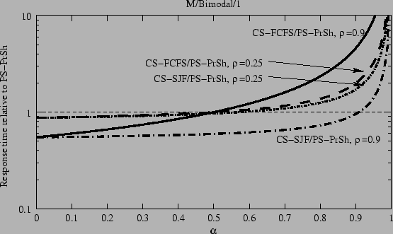
Figure 3.3 shows the average response time for circuit switching (for both CS-SJF and CS-FCFS) with respect to that for PS-PrSh for different values of $\alpha$ and for link loads of 25% and 90%. A value of below 1 indicates a faster response time for circuit switching, a value above 1 shows that packet switching is faster.

Figure 3.3:

The figure is best understood by revisiting the motivating examples in sections 3.3.1 and 3.3.2. When $\alpha$ is small, almost all flows are of size B $\approx$ E[X], and the flow size variance is small, $\sigma_{{X}}^{{2}}$ = (E[X] - A)²×$\alpha$/(1 - $\alpha$) $\ll$ (E[X])². As we saw in the first example, in this case the average waiting times for both CS-FCFS and CS-SJF are about 50% of those for PS-PrSh for high loads.

On the other hand, when $\alpha$ approaches 1, most flows are of size A, and only a few are of size B = (E[X] - $\alpha$A)/(1 - $\alpha$) $\longrightarrow$ $\infty$. Then $\sigma_{{X}}^{{2}}$ = (E[X] - A)²×$\alpha$/(1 - $\alpha$) $\longrightarrow$ $\infty$, and so the waiting time of circuit switching also grows to $\infty$. This case is similar to our second example, where occasional very long flows block short flows, leading to very high response time.

We can determine exactly when CS-FCFS outperforms PS-PrSh based on Equations 3.1 and 3.2. The ratio of their expected waiting time is E[X²]/(2E[X]²), and so as long as the coefficient of variation C² = E[X²]/E[X]² - 1 is less than 1, CS-FCFS always behaves better than PS-PrSh. On the other hand, CS-SJF behaves better than CS-FCFS, as expected, and it is able to provide a faster response time than PS-PrSh for a wider range of flow size variances, especially for high loads when the job queue is often non-empty and the reordering of the queue makes a difference. However, CS-SJF cannot avoid the eventual hogging by long flows when the job-size variance is high, and then it performs worse than PS-PrSh.

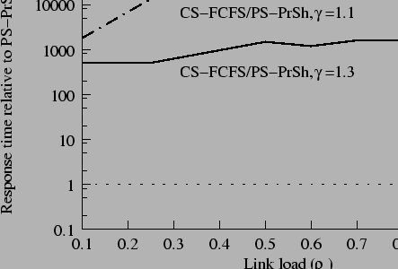
It has been reported [84,57,183] that the distribution of flow durations is heavy-tailed and that it has a very high variance, with an equivalent $\alpha$ greater than 0.999. This suggests that PS-PrSh is significantly better than either of the circuit-switching disciplines. I have further verified this conclusion using a Bounded-Pareto distribution for the flow size, such that f (x) $\propto$ x^-$\gamma$-1. Figure 3.4 shows the results. It should not be surprising how bad circuit switching fares with respect to packet switching given the high variance in flow sizes of the Pareto distribution.

Figure 3.4:

We can conclude that in a LAN environment, where a single end host can fill up all the link bandwidth, packet switching leads to more than 500-fold lower expected response time that circuit switching because of link hogging.