In the previous section, we saw what happens when a circuit belonging to a user flow blocks the link for long periods of time. However, this is not possible in the core of the network. For example, most core links today operate at 2.5 Gbit/s (OC48c) or above [30], whereas most flows are constrained to 56 Kbit/s or below by the access link [59]. Even if we consider DSL, cable modems and Ethernet, when the network is empty a single user flow cannot fill the core link on its own. For this case, we need a different analysis.
For the core of the network, I will consider a slightly modified version of the last example for LANs. Now, client hosts access the network through a 1 Mbit/s link, as shown in Figure 3.5. Again, the transcontinental link has a capacity of 1 Gbit/s, and there are 99 files of 10 Mbits and a single 10-Gbit file. In this case, flow rates are capped by the access link at 1 Mbit/s no matter what switching technology is used. With circuit switching, it does not make sense to allocate a circuit in the core that has more capacity than the access link because the excess bandwidth would be wasted. So, all circuits get 1 Mbit/s, and because the core link is of 1 Gbit/s, all 100 circuits of 1 Mbit/s can be admitted simultaneously. Similarly, we can fit all 100 packet-switched flows of 1 Mbit/s. If there is no difference in the flow bandwidth or the scheduling, then there is absolutely no difference in the response time of both techniques, as shown in Table 3.3. These results are representative of an overprovisioned core network.
0.8!
![\includegraphics[]{fig/TranscontinentalExample3b}](pmf_thesis_img36.png)
|
I will consider a fourth motivating example to illustrate what happens when we oversubscribe the core of the network. Consider the same scenario as before, but with 100 times as many clients and files; namely, we have 10000 clients requesting 9900 files of 10 Mbits and 100 files of 10 Gbits (which get requested slightly before the shorter ones). With circuit switching, all circuits will be of 1 Mbit/s again, and 100 Mbit/s of the core link will be blocked by the long flows for 10000 s, whereas short flows will be served in batches of 900 flows that last 10 s.
With packet switching, all 10000 flows will be admitted, each taking 100 Kbit/s of the core link. After 100 s, all short flows finish, at which point the long flows get 1 Mbit/s until they finish. The long flows are unable to achieve 10 Mbit/s because the access link caps their peak rate. As a result, the average response time for packet switching is 199.9 s vs. the 159.4 s of circuit switching. In addition, the packet-switched system is not longer work conserving, and, as a consequence, the last flow finishes later with packet switching. The key point of this example is that by having more channels than long flows one can prevent circuit switching from hogging the link for long periods of time. Moreover, the oversubscription of a link with flows hurts packet switching because the flow bandwidth is squeezed.
Which of these two scenarios for the core is more representative of the Internet today? I will argue that it is Example 3.4.1 (for which circuit switching and packet switching perform similarly) because it has been reported that core links are heavily overprovisioned [135,47,90].
At the core of the Internet, flow rates are limited by the access link rate, and so a single user cannot block a link on its own. To reflect this, the analytical model of Section 3.3.3 needs to be adjusted by capping the maximum rate that a flow can receive. I will use N to denote the ratio between the data rates of the core link and the access link. For example, when a flow from a 56 Kbit/s modem crosses a 2.5 Gbit/s core link, N = 44, 000. Now, in the fluid model a single flow can use at most 1/N of the whole link capacity, so rather than having a full server, I will use N parallel servers, each with 1/N of the total capacity. In other words, I will use an M/GI/N model instead. For this model, there is an analytical solution for the PS-PrSh discipline [49]; however, there is no simple closed-form solution for CS-FCFS or CS-SJF, so I resort to simulation for these disciplines instead.
With circuit switching, the more circuits that run in parallel, the less likely it is that enough long flows appear at the same time to hog all the circuits. It is also interesting to note that CS-SJF will not necessarily behave better than CS-FCFS all the time, as CS-SJF tends to delay all long jobs and then serve them in a batch when there are no other jobs left. This makes it more likely for hogging to take place, blocking all short jobs that arrive while the batch of long jobs is being served. On the other hand, CS-FCFS spreads the long jobs over time (unless they all arrived at the same time), and it is therefore less likely to cause hogging. For this reason and because of the difficulties implementing CS-SJF in a real network, I will no longer consider it in our M/GI/N model.
|
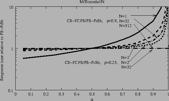
Figure 3.6 compares the average response time for CS-FCFS against PS-PrSh for bimodal service times and different link loads. The ratio, N, between the core-link rate and the maximum flow rate varies from 1 to 512. We observe that as the number of flows carried by the core link increases, the performance of CS-FCFS improves and approaches that of PS-PrSh. This is because for large N the probability that there are more than N simultaneous long flows is extremely small. The waiting time becomes negligible, since all jobs reside in the servers, and so circuit switching and packet switching behave similarly. Figures 3.7a and 3.7b show similar results for bounded Pareto flow sizes as we vary the link load. Again, as N becomes greater or equal to 512, there is no difference between circuit and packet switching in terms of average response time for any link load. I have also studied the standard deviation of the response time,
![]() , for both flow size distributions, and there is also little difference once N is greater than or equal to 512.
, for both flow size distributions, and there is also little difference once N is greater than or equal to 512.
|
To understand what happens when N increases, we can study Figure 3.8. As we can see, the number of flows in the queue (shown in the upper three graphs) increases drastically whenever the number of long jobs in the system (shown in the bottom three graphs) is larger than the number of servers, which causes a long-lasting hogging. Until the hogging is cleared, there is an accumulation of (mainly) short jobs, which increases the response time. As the number of servers increases, the occurrence of hogging events is less frequent because the number of long flows in the system is smaller than the number of servers, N, almost all the time. The results for an M/Bimodal/N system are very similar.
|
In the core, N will usually be very large. On the other hand, in metropolitan networks, N might be smaller than the critical N, at which circuit switching and packet switching have the same response time. Then, in a MAN a small number of simultaneous, long-lived circuits might hog the link. This could be overcome by reserving some of the circuits for short flows, so that they are not held back by the long ones, but it requires some knowledge of the duration of a flow when it starts.
One way of forfeiting this knowledge of the flow length could be to accept all flows, and only when they last longer than a certain threshold, they are classified as long flows. However, this approach has the disadvantage that long flows may be blocked in the middle of the connection.
One might wonder why a situation similar to Example 3.4.2 does not happen. In that example, there were many more active flows than the ratio N, and then the packet-switched flows would squeeze the available bandwidth. However, if we consider Poisson arrivals, the probability that there are at least N arrivals during the duration of a ``short'' flow is very small because most bytes (work) are carried by long flows as shown in Figure 1.6. As a result,
P(at least N arrivals during short flow) = 1 - F![]() (N - 1)
(N - 1) ![]() 0 as
N
0 as
N ![]()
![]() , where
F
, where
F![]() is cumulative distribution function (CDF) of a Poisson distribution with parameter
is cumulative distribution function (CDF) of a Poisson distribution with parameter
![]() , and:
, and:
![]() =
= ![]() ×
×![]() =
= ![]()
![]() ×
×![]() ×N =
×N = ![]() ×
×![]() ×N
×N ![]()
![]() ×N < N
×N < N
where
0 < ![]() < 1 is the total system load,
E[X| short]
< 1 is the total system load,
E[X| short] ![]() E[X] is the average size of short flows, and R is the link capacity. As a result,
P(at least N arrivals during short flow)
E[X] is the average size of short flows, and R is the link capacity. As a result,
P(at least N arrivals during short flow) ![]() 0.
0.
In summary, the response time for circuit switching and packet switching is similar for current network workloads at the core of the Internet, and, thus, circuit switching remains a valid candidate for the backbone. As a reminder, these are only theoretical results and they do not include important factors like the packetization of information, the contention along several hops, the delay in feedback loops, or the flow control algorithms of the transport protocol. The next section explores what happens when these factors are considered.